Lab: QLoRA fine-tune on the caption catalogue. PLO: PLO2 / PLO3. Points: 7.
Overview
The catalogue has 5,000 assets without captions. The unit could prompt a large model every time, retrieve similar captions and let a frozen model copy their shape, or fine-tune a small model on its own catalogue. The one big idea for this session: inference is limited by memory bandwidth, and fine-tuning buys behaviour while retrieval buys knowledge — the choice is about which one the task needs.
The lab makes the trade concrete: a 4-billion-parameter model, a 1,000-row synthetic caption catalogue, and a LoRA adapter trained on a Mac, a free T4 or the faculty RTX Pro 6000. The base model writes fluent marketing copy; the tuned model learns the unit's one-sentence, factual voice.
Lesson
Why inference is memory-bound
A generated token requires reading the model's weights and the KV cache. At batch 1, the arithmetic is small compared with the bytes moved, so the rate is set by memory bandwidth, not by floating-point throughput: roughly tokens/s ≈ bandwidth ÷ bytes moved per token. That is why a 4-bit model can be several times faster than the same model in FP16 on the same chip, and why batching changes the picture — more tokens per weight read raises arithmetic intensity until compute becomes the limit.
The media unit feels this as latency: a caption request that waits 20 seconds is a different product from one that waits 2.
Precision and quantisation
Precision is bytes per parameter. FP16 stores 2 bytes, FP8 stores 1 and FP4 stores 0.5, so the weights' memory bill divides by the same factor. Quantization is the act of rounding weights into that smaller format; it trades a little quality for a lot of memory and bandwidth.
The KV cache does not always shrink with the weights, and it grows with context length and batch size. Long media prompts and multiple captions per call can make the cache, not the weights, the surprise. The lab's 4-bit model fits in about 3 GB of weights but peaks near 4.4 GB on the Mac once the cache and activations are counted, and near 5.8 GB on CUDA during training.
LoRA and QLoRA
Full fine-tuning updates every weight and needs memory for gradients and optimizer state several times the model size. LoRA freezes the base and trains small low-rank matrices — the adapter — so the trainable share is a fraction of a percent. In this lab the CUDA path reports 32.46 million trainable parameters of 4.57 billion (0.71%); the MLX path uses rank 8 rather than 16 and trains roughly half that.
QLoRA combines a 4-bit base, LoRA adapters in higher precision, double quantisation and paged optimizers. That is what makes a 4-billion-parameter fine-tune fit a free 16 GB T4. The adapter is small and portable between runs of the same model, but it is not interchangeable across model families or runtimes: the MLX and CUDA adapters are different files.
A useful decision rule: fine-tune when the gap is behaviour (voice, structure, refusal, classification), retrieve when the gap is knowledge (fresh facts, documents, permissions), and prompt when the task is small enough that neither earns its cost. The research question asks the student to defend that rule with numbers from the lab.
The lab: 4B parameters, 1,000 rows
The catalogue is 800 training rows and 200 validation rows, generated with seed 42. The base and tuned models are scored with token-F1 on held-out rows: a teaching metric that rewards factual overlap and punishes fluent filler, not a judge of style.
The measured MLX path loads the 4-bit model in about 40 seconds, trains 100 iterations in about 7 minutes and peaks at 4.42 GB. The CUDA path is measured on both GPUs: the faculty RTX Pro 6000 trains 100 steps in 219.8 s and peaks at 5.76 GB; a free Kaggle T4 trains the same 100 steps in 855.4 s and peaks at 5.78 GB. The device changes the wall-clock time, not the learning: token-F1 rises from 0.5444 to 0.7746 on the RTX and from 0.5449 to 0.7749 on the T4.
What the numbers do and do not show
Token-F1 can rise while the captions become less readable, and it can miss a factual error that the metric's word overlap happens to reward. The samples matter: read three base and three tuned captions and say what changed. A model that learns the unit's voice but repeats a wrong licence is not a successful fine-tune.
The economics
Training is a one-off cost; inference is the recurring one. A 4-bit adapter makes both smaller. The next session compares the Mac, the T4 and the RTX Pro 6000 on the same task, so this session records the time and memory that make that comparison possible.
Check yourself
Why can a 4-bit model generate faster than the same model in FP16, and what limits the gain?
What does LoRA freeze, and why does that make the fine-tune fit a 16 GB card?
A client asks for captions in a new brand voice, and the product list changes every week. Which do you fine-tune, and which do you retrieve?
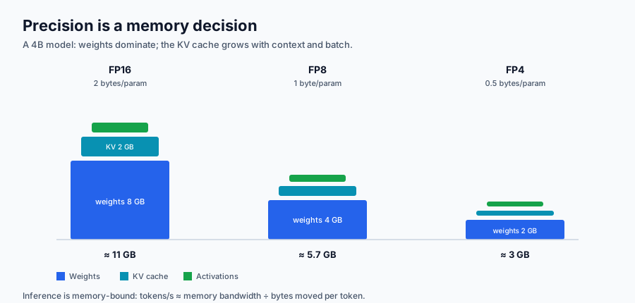
The scene shows the same 4-billion-parameter model at FP16, FP8 and FP4. Switch precision and watch the weights, KV cache and activations change height. The totals are teaching estimates for a 4B model; the lab records the measured peak.
The stack in words. Weights dominate the memory bill: 8 GB at FP16, 4 GB at FP8 and 2 GB at FP4 for a 4B model. The KV cache adds 2, 1 and 0.5 GB, and activations add about 1, 0.7 and 0.5 GB. The totals are about 11, 5.7 and 3 GB. Fewer bytes per parameter means fewer bytes moved per token, which is why quantization raises throughput until compute or the cache takes over.
Mode
Bytes/param
Weights
KV cache
Activations
Approx. total
FP16
2.0
8.0 GB
2.0 GB
1.0 GB
11.0 GB
FP8
1.0
4.0 GB
1.0 GB
0.7 GB
5.7 GB
FP4
0.5
2.0 GB
0.5 GB
0.5 GB
3.0 GB
The table is the same information as the scene; the lab measures the real peak, which includes framework overhead and the adapter.
Prerequisite: A phone-verified Kaggle account, or an Apple-silicon Mac with the kit's S9 dependency group; internet access for Kaggle's install cell. Set it up in Session 0: Accounts, Tools, The kit.
Lab — QLoRA fine-tune on the caption catalogue
Time: 120 minutes — 15 setup, 60 fine-tune, 25 evaluate, 10 evidence, 10 teardown. On the Mac the full run is about 15 minutes; on a free Kaggle T4 the measured full run is about 18 minutes end to end (14.3 min training + ~2 min load/eval) at 5.78 GB peak VRAM; on the faculty RTX Pro 6000 Blackwell it is about 4.5 minutes (3.7 min training + ~40 s load/eval) at 5.76 GB. Start the smoke run first so the full run is not the first time you meet the runtime.
Prerequisite: S8; Python 3.14; basic ML vocabulary. The data is bundled at data/caption_catalogue.jsonl — 1,000 synthetic rows, 800 train / 200 validation, course-owned, seed 42. The provenance, licence and fetch instructions are in data/README.md; there is no runtime download.
You need to know: at batch 1, inference is memory-bound; precision divides the weights' memory bill; LoRA freezes the base and trains a small adapter; QLoRA adds a 4-bit base and memory-saving optimizer tricks.
Safe-data acknowledgement: I have read the lab safe-data policy. I will use only the course-supplied synthetic media and will not upload real personal media to any cloud service.
Task
Fine-tune a 4-bit QLoRA adapter on the synthetic caption catalogue, compare the base and tuned captions with token-F1 on held-out rows, and explain when this beats prompting or retrieval.
Mac. Open notebook.ipynb. The install cell (the single documented pip install exception) checks imports first: in the course environment the MLX stack is already there, so it prints already installed — nothing to do and installs nothing. If you built the environment by hand it installs mlx==0.32.4, mlx-metal==0.32.4 and mlx-vlm[train]==0.7.12 once; restart the kernel after that run. For the smoke run, start the kernel with the two documented overrides — export them in the terminal you launch JupyterLab from, or edit the S9_ITERS and S9_EVAL_ROWS defaults in the configuration cell:
export S9_ITERS=2 S9_EVAL_ROWS=2 # smoke run; unset both (or use 100 and 10) for the full run
Then run the cells from the import cell down.
Kaggle. Create a private notebook and attach the catalogue as a private dataset. The notebook searches /kaggle/input for caption_catalogue.jsonl, so the dataset name and Kaggle's mount layout do not matter; to be explicit, set COURSE_DATA to the folder that contains the file. Set Accelerator → GPU T4 ×2 (the notebook puts the model on one 16 GB GPU). Open notebook-cuda.ipynb, turn Internet on for the install cell, run it, restart the kernel, and set ITERS=10, EVAL_ROWS=5 for the smoke run.
Faculty RTX. Use the same CUDA notebook; the training stack may already be installed. Confirm the GPU with nvidia-smi before starting.
Console/UI checks:
# Kaggle: Settings → Accelerator shows GPU T4 x2; Internet is ON for the install cell.
# Faculty RTX / RunPod:
nvidia-smi
python3 -c "import torch; print(torch.cuda.get_device_name(0))"
Record the GPU name, the smoke time and the peak memory. If the smoke run's loss does not fall, stop and diagnose before the full run.
2. Run the full fine-tune
Restore the full settings (ITERS=100, EVAL_ROWS=20 on CUDA; 100 and 10 on MLX) and run from the data cell down. The notebook prints the loss every ten steps and writes the result JSON.
Mac:results/mlx_results.json.
CUDA:results/cuda_results.json.
Record the training time, evaluation time and peak memory. The expected MLX peak is about 4–5 GB; the measured CUDA peak is 5.8 GB on both the T4 and the RTX card, well under the T4's 15.6 GB. The measured 100-step T4 run takes 855 s; if your session is slower, set ITERS=50. If it runs out of memory, keep MAX_SEQ_LEN=512 and batch 1, and rely on gradient accumulation.
3. Evaluate and read the samples
The notebook computes token-F1 for the base and the tuned model on the same held-out rows. Build the base-vs-tuned table:
Model
Token-F1
Seconds
Peak memory
Base
Tuned
Read three sample captions from the JSON. Say what the base got wrong and what the tuned model changed. Token-F1 is a teaching metric; it does not judge style, and it can miss a factual error.
4. Explain the choice
Write 150–250 words: when would this fine-tune beat retrieval over a larger frozen model, and when would retrieval win? Use your numbers — training time, adapter size, inference speed, update cost — and name one thing the unit would need to redo when the product list changes. This is the lab half of the research question.
5. Save the evidence and tear down
Copy the result JSON and the three samples out of the notebook before the session ends. On Kaggle, stop the session; the output is not a durable store. On RunPod, terminate the pod and its network volume; the container disk clears on stop but a network volume persists.
Evidence bundle
The result JSON (mlx_results.json or cuda_results.json) with runtime, model, time, peak memory and base/tuned F1.
The base-vs-tuned table and three sample captions.
A three-sentence what this proves note: what the base got wrong, what the tuned model changed, and why LoRA is cheaper than full training.
A 150–250 word fine-tune-versus-retrieval argument with your numbers.
A teardown log: session stopped or pod and volume terminated, adapter and outputs copied or deleted, GPU confirmed idle.
The bundle is scored 3/2/1/0.
Failure and recovery
The deliberate failure is the memory wall: on a 16 GB T4, raise MAX_SEQ_LEN to 1024 (or batch_size above 1) and watch it run out of memory. Recover by returning to MAX_SEQ_LEN=512, batch 1, gradient accumulation and ITERS=100 (or 50 if time is short). On the Mac, the same experiment with a larger sequence or batch shows the unified-memory limit; keep grad_checkpoint=True and the 4-bit model. The lesson is that the memory budget, not the parameter count alone, sets the feasible configuration.
If the loss stalls or the model diverges: confirm the chat template strips thinking, check that train_on_completions is on, lower the learning rate, and compare a base sample to a tuned sample rather than trusting one scalar.
Cost ceiling
$0 on this Mac, the free Kaggle T4 and the faculty RTX Pro 6000. A RunPod fallback stays under $3.40 at $1.69/hr for two hours; set S9_HOURLY_COST in the CUDA notebook to record the line. There is no persistent storage in the lab beyond the result JSON.
Teardown
Mac: delete the adapter and the results/ folder after copying the JSON; confirm no process is using the GPU.
Kaggle: stop the session; download the result JSON and samples first.
Faculty RTX: stop the kernel; remove the adapter and outputs from the shared workspace.
RunPod: terminate the pod and the network volume; confirm the billing page shows no running instance.
Fallback
If the runtime cannot complete the fine-tune, use the precomputed prototype results in prototypes/ai-inference-finetuning/results/ (t4_smoke.json, t4_full.json, rtx_pro_6000_*.json) and run the evaluation on the base model only; the evidence shape is unchanged but the note must say which row is measured and which is cited. If the 4B model does not fit, use Qwen3.5-2B and record the change. The T4 smoke run is the gate and has been verified; if a student's session fails, use the Mac MLX path or the faculty RTX card.
Each document name opens a rendered view you can read in the browser. The download link beside it gives you the raw Markdown working file: the copy you edit, run and submit. The page above and the lab steps carry the teaching.
The runnable notebook that produces the lab's numbers.
Research question
For a small media team with domain data, when does a small fine-tuned model beat retrieval over a larger frozen model?
Submit an 800–1,200 word answer with 5–8 sources at the next session. The rubric and the exemplar guidance show the expected shape.
References — Session 9
Hu, E. J., Shen, Y., Wallis, P., Allen-Zhu, Z., Li, Y., Wang, S., Wang, L., & Chen, W. (2022). LoRA: Low-rank adaptation of large language models. International Conference on Learning Representations (ICLR). https://arxiv.org/abs/2106.09685
Makes fine-tuning a small model affordable by training low-rank adapters instead of all weights — the method the lab uses. Adapter capacity and rank selection for multimodal media tasks are still empirical. The LoRA adapter diagram needs a redraw or permission.
Dettmers, T., Pagnoni, A., Holtzman, A., & Zettlemoyer, L. (2023). QLoRA: Efficient finetuning of quantized LLMs. Advances in Neural Information Processing Systems 36. https://arxiv.org/abs/2305.14314
Shows how 4-bit quantisation plus LoRA fits a useful model into a free T4, which is the lab's constraint. The quality cost of 4-bit fine-tuning on small domain datasets is task-dependent and under-reported. The memory diagram is a redraw candidate.
Lewis, P., Perez, E., Piktus, A., et al. (2020). Retrieval-augmented generation for knowledge-intensive NLP tasks. Advances in Neural Information Processing Systems 33. https://arxiv.org/abs/2005.11401
The alternative to fine-tuning: keep the model frozen and supply documents, which changes cost, freshness and governance. RAG versus fine-tuning for media-domain knowledge has no settled cost model. The RAG pipeline can be rebuilt as a node-graph scene.
Kaplan, J., McCandlish, S., Henighan, T., et al. (2020). Scaling laws for neural language models. arXiv:2001.08361. https://arxiv.org/abs/2001.08361
Explains why model size, data and compute trade against each other — the numbers behind the week's memory-bandwidth discussion. Scaling laws for small, domain-specific models and inference-optimised architectures are less clear. The loss curves can be redrawn from the reported data.
Teaching note. Narrate Hu et al. (2022) for 5–8 minutes, assign the abstract of Dettmers et al. (2023) as reading, and close by restating the open problem as the weekly question. Figures are third-party; redraw by default.
PLO — Session 9: LLM inference and fine-tuning
CLO: By the end of this session, the student can explain why inference is memory-bound, fine-tune a 4-bit QLoRA adapter on a small catalogue, and defend a choice between fine-tuning, retrieval and prompting with measured time and token-F1.
PLO
Role
Research answer
Lab evidence
Points
Evidence
Rubric
PLO2
primary
4
3
7
An 800–1,200-word fine-tune-versus-retrieval argument with 5–8 sources; the results JSON, base-vs-tuned table, three samples, the cost note and the teardown
Research 4/3/2/1; Lab 3/2/1/0
PLO3
secondary
0
0
0
Lecture context only; not scored
—
Total
4
3
7
Total: 7 points
Four-level descriptors
Research (4/3/2/1). 4 = a decision rule that separates behaviour from knowledge, applied to the unit's captioning task with measured time, memory and token-F1; cost, latency, update cadence and privacy compared; a counterargument (retrieval is cheaper to update) weighed. 3 = a sound rule with the lab numbers and some comparison. 2 = describes fine-tuning and RAG without choosing or using measurements. 1 = a summary with fewer than five sources. 0 = nothing submitted or misconduct.
Lab (3/2/1/0). 3 = the smoke and full runs complete, the result JSON records runtime, time, peak memory and base/tuned F1, the samples are read and explained, the fine-tune-versus-retrieval argument uses the numbers, and teardown is complete. 2 = mostly complete, one check thin. 1 = a partial run or an unrecorded measurement. 0 = nothing submitted, unsafe data, or no teardown.
The full course arithmetic is in production/baseline.md; this file is the weekly instance.